How To Find Opportunity Cost From A Graph

Step 1. The equation for any budget constraint is the post-obit:

[latex]\text{Budget }={P}_{ane}\times{Q}_{1}+{P}_{2}\times{Q}_{2}+\dots+{P}_{northward}\times{Q}_{north}[/latex]

where P and Q are the toll and respective quantity of any number, northward, of items purchased and Budget is the corporeality of income one has to spend.

Step 2. Apply the upkeep constraint equation to the scenario.

In Charlie's case, this works out to be

[latex]\begin{array}{l}\text{Budget}={P}_{one}\times{Q}_{1}+{P}_{2}\times{Q}_{two}\\\text{Budget}=\$ten\\\,\,\,\,\,\,\,\,\,\,\,\,{P}_{i}=\$2\left(\text{the cost of a burger}\correct)\\\,\,\,\,\,\,\,\,\,\,\,\,{Q}_{ane}=\text{quantity of burgers}\left(\text{variable}\right)\\\,\,\,\,\,\,\,\,\,\,\,\,{P}_{2}=\$0.50\left(\text{the price of a motorbus ticket}\right)\\\,\,\,\,\,\,\,\,\,\,\,\,{Q}_{two}=\text{quantity of tickets}\left(\text{variable}\correct)\end{array}[/latex]

For Charlie, this is

[latex]{\$10}={\$2}\times{Q}_{one}+{\$0.50}\times{Q}_{two}[/latex]

Step 3. Simplify the equation.

At this point we need to decide whether to solve for [latex]{Q}_{1} [/latex] or [latex]{Q}_{2} [/latex].

Remember, [latex]{Q}_{i} = \text{quantity of burgers} [/latex]. So, in this equation [latex]{Q}_{one} [/latex] represents the number of burgers Charlie can purchase depending on how many bus tickets he wants to buy in a given week. [latex]{Q}_{two}=\text{quantity of tickets} [/latex]. So, [latex]{Q}_{2} [/latex] represents the number of bus tickets Charlie can purchase depending on how many burgers he wants to purchase in a given week.

Nosotros are going solve for [latex]{Q}_{1} [/latex].

[latex]\begin{assortment}{l}\,\,\,\,\,\,\,\,\,\,\,\,\,\,\,\,\,\,\,\,10=2Q_{1}+0.50Q_{2}\\\,\,\,x-2Q_{1}=0.50Q_{2}\\\,\,\,\,\,\,\,\,\,\,\,\,-2Q_{1}=-10+0.50Q_{two}\\\left(2\correct)\left(-2Q_{1}\right)=\left(two\right)-10+\left(ii\correct)0.50Q_{2}\,\,\,\,\,\,\,\,\,\text{Clear decimal past multiplying everything by 2}\\\,\,\,\,\,\,\,\,\,\,\,\,-4Q_{ane}=-20+Q_{2}\\\,\,\,\,\,\,\,\,\,\,\,\,\,\,\,\,\,\,\,Q_{1}=5-\frac{i}{four}Q_{2}\,\,\,\,\,\,\,\,\,\,\,\,\,\,\,\,\,\,\,\,\,\,\,\,\,\,\,\,\,\,\,\,\,\,\,\,\,\,\,\,\text{Divide both sides past}-four\end{array}[/latex]

Step four. Use the equation.

Now we have an equation that helps us calculate the number of burgers Charlie can purchase depending on how many motorcoach tickets he wants to buy in a given week.

For example, say he wants viii jitney tickets in a given week. [latex]{Q}_{2}[/latex] represents the number of coach tickets Charlie buys, so we plug in 8 for [latex]{Q}_{2}[/latex], which gives us

[latex]\begin{array}{fifty}{Q}_{ane}={5}-\left(\frac{1}{4}\right)viii\\{Q}_{1}={five}-2\\{Q}_{one}=3\end{assortment}[/latex]

This means Charlie tin can buy 3 burgers that calendar week (point C on the graph, higher up).

Permit'southward attempt i more. Say Charlie has a calendar week when he walks everywhere he goes so that he can splurge on burgers. He buys 0 bus tickets that week. [latex]{Q}_{2}[/latex] represents the number of bus tickets Charlie buys, so nosotros plug in 0 for [latex]{Q}_{2}[/latex], giving us

[latex]\begin{array}{fifty}{Q}_{1}={v}-(\frac{one}{4})0\\{Q}_{1}={5}\end{array}[/latex]

And so, if Charlie doesn't ride the omnibus, he can buy five burgers that week (point A on the graph).

If you plug other numbers of bus tickets into the equation, you get the results shown in Table one, beneath, which are the points on Charlie'southward budget constraint.

Table 1.
Point	Quantity of Burgers (at $2)	Quantity of Bus Tickets (at fifty cents)
A	5	0
B	iv	4
C	3	eight
D	ii	12
E	1	sixteen
F	0	xx

Step v. Graph the results.

If we plot each point on a graph, we can come across a line that shows us the number of burgers Charlie can purchase depending on how many bus tickets he wants to buy in a given week.

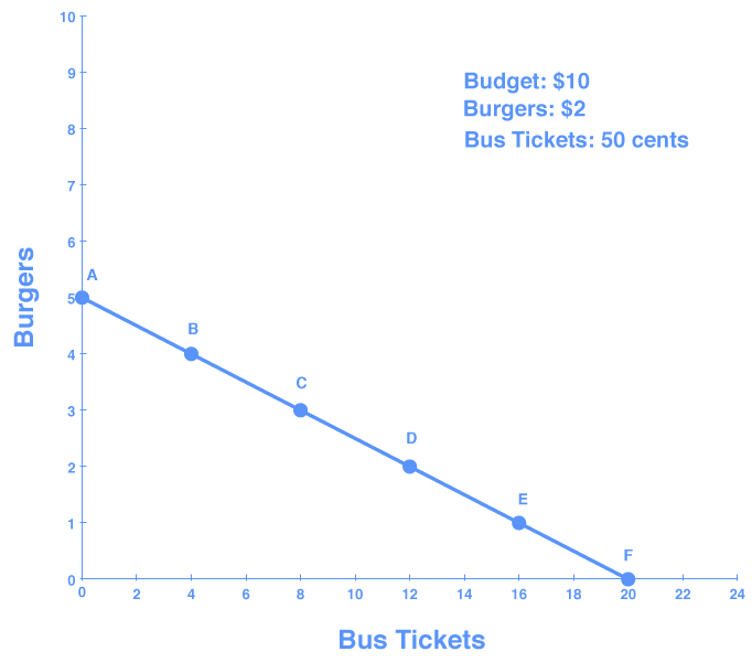
Graph showing budget line as a downward slope representing the opportunity set of burgers and bus tickets. The line starts at 0,5 and ends at 20,0.

Effigy 2. Charlie'due south Budget Constraint.

Nosotros can make two important observations most this graph. First, the slope of the line is negative (the line slopes down from left to right). Remember in the concluding module when we discussed graphing, we noted that when when X and Y have a negative, or inverse, human relationship, Ten and Y move in opposite directions—that is, as one rises, the other falls. This ways that the merely way to become more of ane good is to give up some of the other.

Second, the gradient is divers as the alter in the number of burgers (shown on the vertical centrality) Charlie tin can purchase for every incremental alter in the number of tickets (shown on the horizontal centrality) he buys. If he buys i less burger, he can buy 4 more than charabanc tickets. The slope of a budget constraint e'er shows the opportunity cost of the good that is on the horizontal centrality. If Charlie has to requite up lots of burgers to buy just ane passenger vehicle ticket, then the slope will be steeper, considering the opportunity cost is greater.

This is easy to see while looking at the graph, only opportunity cost can also be calculated simply past dividing the toll of what is given up by what is gained. For instance, the opportunity cost of the burger is the cost of the burger divided by the price of the bus ticket, or